Lab 8: Spectral Signature Analysis and Resource Monitoring

Goal

This lab is intended for familiarization with measuring and interpolating spectral signatures, or levels of spectral reflectance, based on imagery collected via satellite. These techniques can also be applied to monitor Earth resources through utilization of remote sensing band ratio techniques.

Background

Part one will introduce how to collect spectral signatures, graph their reflectance, and analyze the remotely sensed images based on the spectral separability test.

Part two will cover vegetation and soils analysis.

Methods

Part 1: Spectral Signature Analysis

We will be using Landsat ETM+ imagery to collect and analyze spectral signatures of Earth surface/near surface features of the Eau Claire and surrounding areas within Wisconsin and Minnesota.

Spectral channel (band) in micrometers in the order of highest reflectance and lowest reflectance for various surface types (screenshot figures seen below)

Signature 1: Standing Water 0.4 micrometers, 0.7 micrometers (figure 1)

Sig 2: Moving Water 0.5 micrometers, 0.7 micrometers (figure 2)

Sig 3: Deciduous Forest 0.6 micrometers, 0.7 micrometers (figure 3)

Sig 4: Evergreen/Coniferous Forest 0.6 micrometers, 0.7 micrometers (figure 4)

Sig 5: Riparian Vegetation 1.3 micrometers, 0.7 micrometers (figure 5)

Sig 6: Crops 0.5 micrometers 1.3 micrometers (figure 6)

Sig 7: Dry Soil 0.7 micrometers, 1.3 micrometers (figure 7)

Sig 8: Moist Soil 0.7 micrometers, 1.3 micrometers (figure 8)

Sig 9: Rock 1.3 micrometers, 0.7 micrometers (figure 9)

Sig 10: Asphalt Highway 0.4 micrometers, 1.3 micrometers (figure 10)

Sig 11: Airport Runway 0.7 micrometers, 1.3 micrometers (figure 11)

Sig 12: Concrete Surface 0.7 micrometers, 0.6 micrometers (figure 12)

Reasons behind signatures:

Absorptance of energy in calm water bodies increases as you get closer to the NIR band, so standing water would have the highest reflectance in the blue band (furthest visible energy from NIR), and lowest reflectance in the red band (closest to NIR of visible wavelengths.) Also, the blue band displays vegetation incorrectly. It needs to be lower than green band to show higher reflectance in blue due to atmospheric interference. (not corrected for atmospheric scattering)

Deciduous forests display the highest and lowest reflectance at the spectral channels of 0.7 and 0.6 micrometers, respectively. Deciduous forests (figure 3) have different leaf structures that reflect more energy than coniferous (figure 4) leaf structures. There is also a higher leaf area to stem-branch ratio in dorsiventral leaves compared to the needle-leafed conifer. Broad leaves reflect up to 10% more than needle-leaves.

The spectral channel that dry (figure 7) and moist (figure 8) soil vary the most within is the 0.6 micrometer channel, or the range between green and red channels. The difference is due to the change in soil moisture content between moist and dry soils. The drier a soil is, the more reflective it is. The more moisture a soil has, the less reflective it is. The channel that shows the most difference between the two soil types is the red channel. (figure 13)

Part 2: Resource Monitoring

Section 1: Vegetation Health Monitoring

We used band ratios to monitor health of vegetation and soils from remotely sensed images.

Through use of the unsupervised -> indices tool from the Raster Classification tab, we are able to single out areas with vegetation and without.

The presence or absence of vegetation in areas that are medium gray and black represents areas with little to no vegetation, and/or water features. Water has no reflectance in the NDVI (normalized difference vegetation index) image, thus it shows up as black. Medium gray shows healthy vegetation with more moisture. (Figure 15)

NDVI: NIR-Red/NIR+Red

Section 2: Soil Health Monitoring

Most of the ferrous minerals seem to be concentrated in the west and south west portions of Chippewa and Eau Claire counties. However, there are many plots throughout the two counties that show a dispersal of ferrous minerals amongst non-exposed soil and vegetated areas in the north and east of the study area. (Figure 16)

Ferrous Mineral: MIR/NIR

Results

Figure 1 Standing Water Signature Mean Plot Highest reflectance band: 0.4 micrometers Lowest reflectance band: 0.7

Figure 2 Moving Water Signature Mean Plot Highest reflectance band: 0.4 Lowest reflectance band: 1.3

Figure 3 Deciduous Forest Signature Mean Plot Highest reflectance band: 0.7 Lowest reflectance band: 0.6

Figure 4 Evergreen Forest Signature Mean Plot Highest reflectance band: 1.3 Lowest reflectance band: 0.6

Figure 5 Riparian Vegetation Signature Mean Plot Highest reflectance band: 0.4 Lowest reflectance band: 3.0

Figure 6 Crops Signature Mean Plot Highest reflectance band: 1.3 Lowest reflectance band: 0.6

Figure 7 Dry Soil Signature Mean Plot Highest reflectance band: 0.7 Lowest reflectance band: 1.3

Figure 8 Moist Soil Signature Mean Plot Highest reflectance band: 1.3 Lowest reflectance band: 0.7

Figure 9 Rock Signature Mean Plot Highest reflectance band: 1.3 Lowest reflectance band: 0.7

Figure 10 Asphalt Highway Signature Mean Plot Highest reflectance band: 1.3 Lowest reflectance band: 0.7

Figure 11 Airport Runway Signature Mean Plot Highest reflectance band: 1.3 Lowest reflectance band: 0.7

Figure 12 Concrete Surface Signature Mean Plot Highest reflectance band: 0.6 Lowest reflectance band: 0.7

Figure 13 Spectral Profile of Dry vs Moist Soil  Largest gap between the two signatures occurs at 0.6 micrometers.

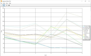
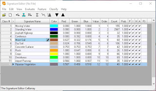
Figure 14 All Spectral Signatures for Each of the 12 Surface Features and Key

Figure 15 The areas with very white values in the NDVI image should represent areas with little vegetation.

Figure 16 The areas with more red areas represent soils with higher concentrations of ferrous minerals.

Sources

Satellite image is from Earth Resources Observation and Science Center, United States Geological Survey.